SINDy Module

Discover the equations hidden in your data

Desiring a more expedited approach to formulating mathematical laws from experimental observations?

The problem: you have raw measurements, but no known differential equation describing how the system evolves.

Sparse Identification of Nonlinear Dynamics (SINDy) searches a library of candidate functions and keeps only the sparsest, cleanest combination that explains your data — turning a CSV file into a governing ODE.

1

Raw data

x(t), state matrix

2

Feature library

Θ(X): Polynomial, Fourier

3

Sparse regression

STLSQ, threshold λ

4

Governing ODE

dx/dt = Δ

Interpretable

Output is a real equation, not a black-box weight matrix — every term has a physical meaning.

Data-driven

No prior knowledge of the underlying physics required — only measurements of the system's states.

Sparse

Thresholded regression prunes weak terms, favoring the simplest equation that still fits.

A real result

From a coupled spring-mass CSV to this, automatically

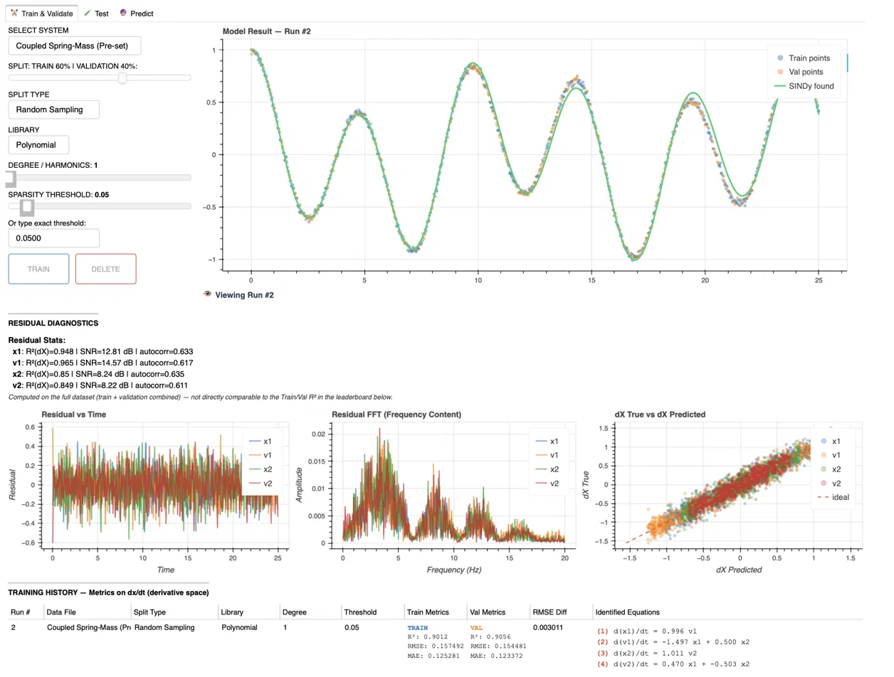
Below is what the module actually recovered from noisy trajectory data — no equation was given to it beforehand.

d(x₁)/dt = 0.996 v₁

d(v₁)/dt = -1.497 x₁ + 0.500 x₂

d(x₂)/dt = 1.011 v₂

d(v₂)/dt = 0.470 x₁ - 0.503 x₂

Validation R² between 0.90 and 0.97 across all four states — with only the correct terms surviving thresholding.

Train tab showing SINDy fit against noisy trajectory data

Output of the Train & Validate tab on the coupled spring-mass system.


About SINDy

Suppose we have a set of measurements \( x(t) \in \mathbb{R}^n \) from some physical system at different points in time \( t \). SINDy seeks to represent the time evolution of \( x(t) \) in terms of a nonlinear function \( f \):

\[ \frac{d}{dt}x(t) = f(x(t)) \]

The key idea behind SINDy is that \( f \) is often sparse in the space of an appropriate set of basis functions — meaning only a small number of terms are nonzero.

For this module, we use Python's pySINDy package to implement SINDy.

Read PySINDy Docs ↗

The Approximation Problem

Data are aggregated into matrices \( X \) and \( \dot{X} \), then a library matrix \( \Theta(X) \) is formed whose columns consist of candidate basis functions:

\[ X = \begin{bmatrix} x_1(t_1) & \dots & x_n(t_1) \\ \vdots & \ddots & \vdots \\ x_1(t_m) & \dots & x_n(t_m) \end{bmatrix}, \quad \dot{X} = \begin{bmatrix} \dot{x}_1(t_1) & \dots & \dot{x}_n(t_1) \\ \vdots & \ddots & \vdots \\ \dot{x}_1(t_m) & \dots & \dot{x}_n(t_m) \end{bmatrix} \]
\[ \Theta(X) = \begin{bmatrix} | & | & & | \\ \theta_1(X) & \theta_2(X) & \dots & \theta_\ell(X) \\ | & | & & | \end{bmatrix} \]

The Core SINDy Problem

SINDy seeks a set of sparse coefficient vectors collected into a matrix \( \Xi \), solving:

\[ \dot{X} \approx \Theta(X)\Xi \]

Each column \( \xi_i \) of \( \Xi \) represents the coefficients for the \( i \)-th component of the model. SINDy uses sparse regression to ensure the resulting model is both accurate and parsimonious — using the simplest possible form.

For example, a sparse \( f(x) \) might look like:

\[ \frac{d}{dt}x = \begin{bmatrix} 1 - x_1 + 3x_1x_2 \\ x_2^2 - 5x_1^3 \end{bmatrix} \]

Built-in systems

The presets are small, noisy time-series datasets chosen to show how library design changes what SINDy can discover. Each training file has two held-out test trajectories from different initial conditions, so you can check whether the recovered equations generalize beyond the fitted data.

Coupled spring–mass system

Two interacting masses exchange energy through linear spring forces.

Linear dynamics 4 states Best first example
Variables
x1, v1, x2, v2
Start with
Polynomial library, degree 1
Research idea
Check whether SINDy keeps only cross-coupled position and velocity terms.
x1' = v1    x2' = v2
v1', v2' = sparse linear combinations of x1 and x2
Van der Pol oscillator

A self-sustained nonlinear oscillator whose trajectories approach a stable limit cycle.

Nonlinear dynamics 2 states Limit cycle
Variables
x, v
Start with
Polynomial library, degree 3
Research idea
Observe why the cubic interaction term is needed to recover the nonlinear damping.
x' = v
v' = -x + μ(1 - x²)v

Nonlinear pendulum

The restoring force is trigonometric rather than polynomial, especially at larger angles.

Periodic dynamics 2 states Trigonometric term
Variables
theta, omega
Start with
Combined library, degree/harmonics 1
Research idea
Compare a polynomial approximation with a library that can represent sin(theta).
theta' = omega
omega' ≈ -sin(theta)

Time-forced oscillator

External periodic forcing is represented by adding time as a state variable named tau.

Time-dependent Augmented state External forcing
Variables
x, tau
Start with
Combined library, degree/harmonics 1
Research idea
See how augmenting time converts a non-autonomous equation into a SINDy-compatible system.
x' ≈ -x + sin(tau)
tau' ≈ 1

Suggested workflow: begin with the recommended library, train the model, inspect the validation metrics and residual plots, then open Test to evaluate the two held-out trajectories. Coefficients may vary slightly with noise, split strategy and sparsity threshold; prioritize a stable sparse structure over matching every coefficient exactly.

Data Source

Bringing In Your Data

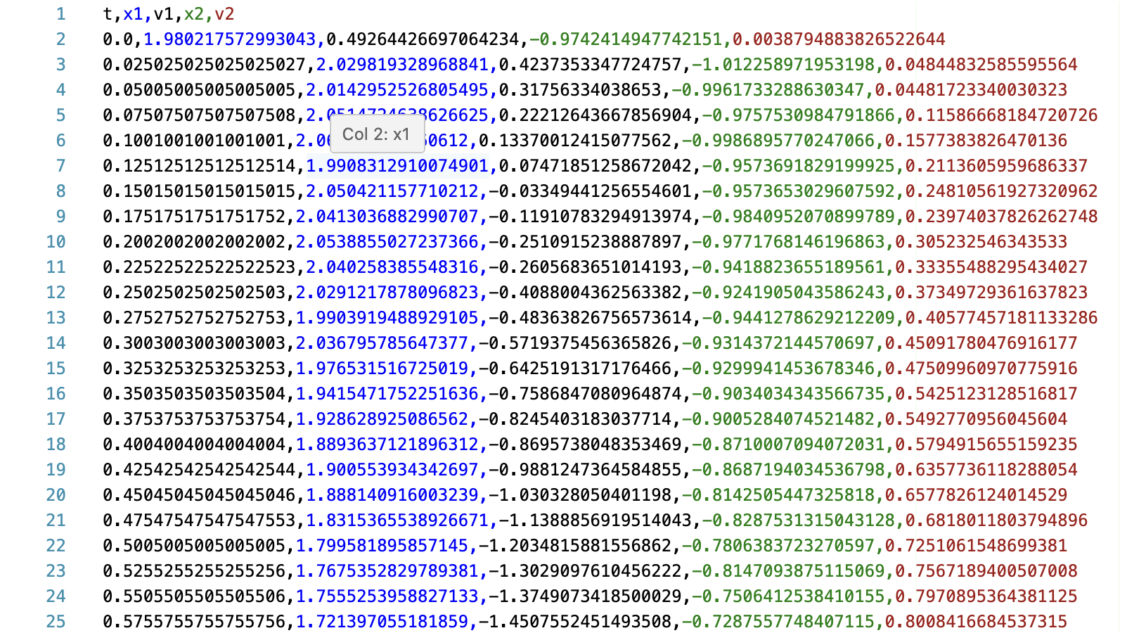
Start from the Select System dropdown. Pick one of the pre-set systems to test SINDy's ability or upload your own data file. The file must have time in the first column and one state variable per subsequent column — \( t, x_1, x_2, \dots, x_n \).

You can upload multiple files when they describe the same state variables under different initial conditions. Every trajectory is validated and differentiated independently, so a time reset between files does not create an artificial derivative jump.

Example of a correctly formatted state-space CSV

A correctly formatted state-space CSV — time in column 1, states after it.


Model Configuration

Choosing How SINDy Learns

Train/Validation set up & Split Strategy

Derivatives \( \dot{X} \) are always computed once on the full trajectory first — the split only decides how the resulting \( (X, \dot{X}) \) pairs are divided afterward. Three strategies are available, and they test different things:

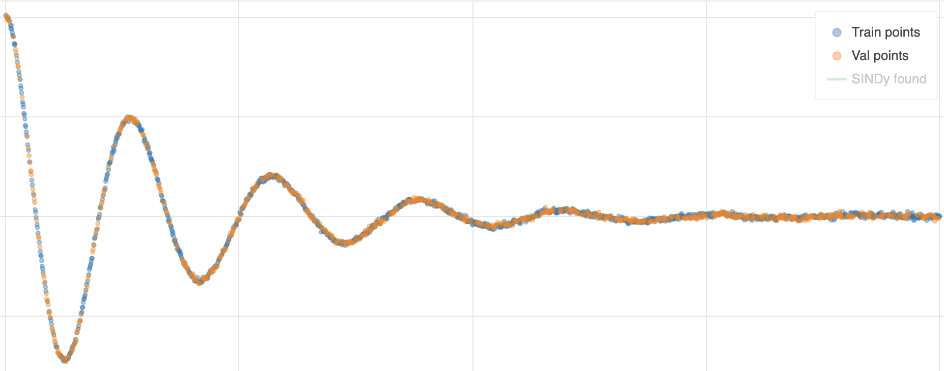
Random Sampling

Every point is shuffled independently into train or validation.

Random Sampling split example

Random Sampling example.

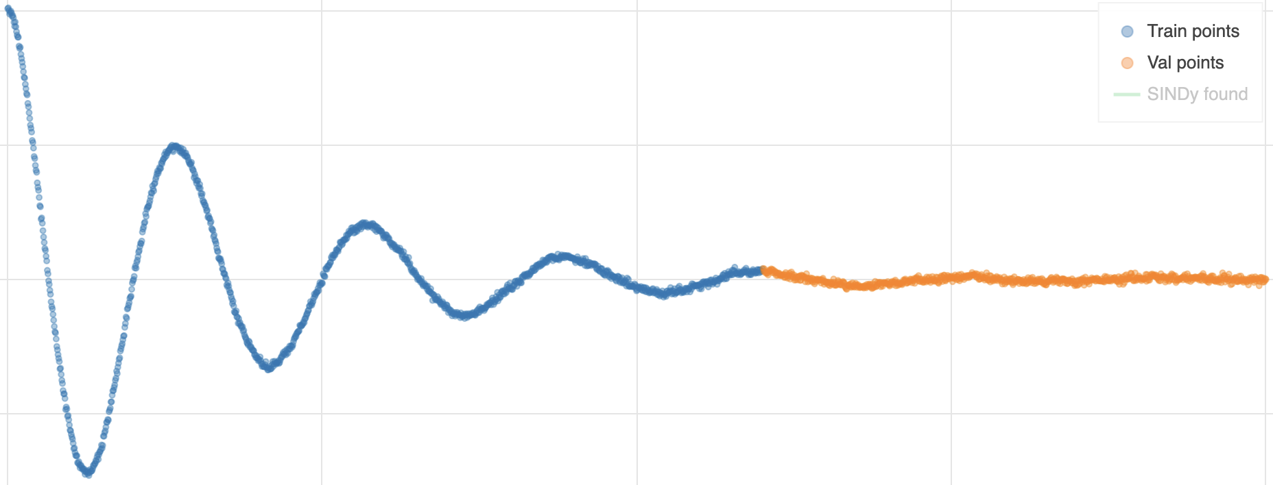
Time-based

Training uses the earlier portion of the trajectory, validation the later portion.

Time-based split example

Time-based example.

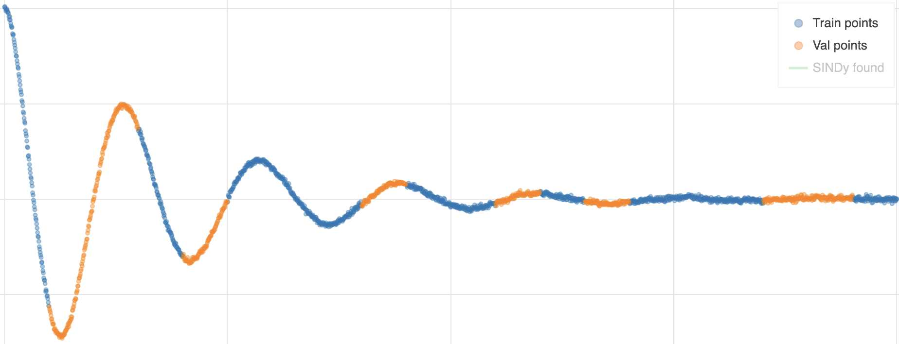
Random Block

Splits by contiguous random blocks instead of single points.

Random Block split example

Random Block example.

Library, degree, and sparsity threshold

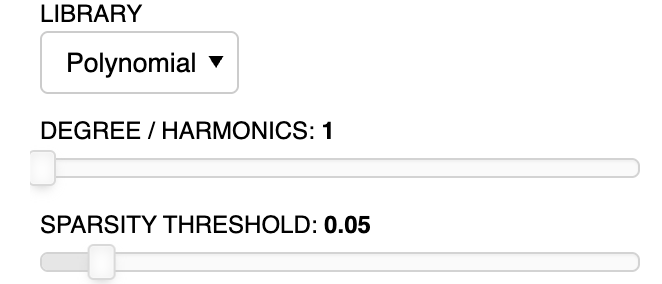
The Library dropdown sets the candidate function space: Polynomial, Fourier, or Combined (both at once).

Degree / Harmonics controls how high the polynomial power (or Fourier harmonic) goes.

The Sparsity Threshold \( (\lambda) \) prunes small coefficients: higher \( \lambda \) means a simpler, sparser equation.

These controls are intentionally selected by the researcher. Compare multiple runs and verify each configuration using validation metrics, residuals, simulation behavior, and domain knowledge.

Hyperparameter controls

SINDy's hyperparameters.


Training Results

Reading the Leaderboard

Every time you press Train, a new row is appended below, so you can compare configurations side by side. Clicking a row to view the run's chart.

Column Meaning
Data File / Split Type Run context: Dataset and Split strategy.
Library / Degree / Threshold Configuration used.
Train/Validation Metrics \( R^2 \), RMSE, and MAE on the training vs. validation split — computed on \( \dot{X} \).
RMSE Diff \( | \text{RMSE}_{\text{train}} - \text{RMSE}_{\text{val}} | \). A large gap is an early warning sign of overfitting.
Identified Equations The actual sparse ODE system SINDy recovered.
History Leaderboard

A run's statistics are record after training.


Model Diagnosis

Residual Diagnostics

A residual is simply the leftover error the model didn't explain: for each state variable, \( \text{residual} = \dot{x}_{\text{true}} - \dot{x}_{\text{predicted}} \), computed across the full dataset.

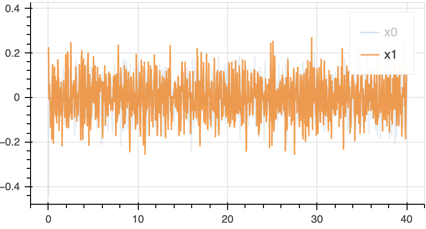
Residual vs. time

A well-fit model's residuals should scatter randomly around zero with no visible trend.

Residual vs .time example

Residual vs time example.

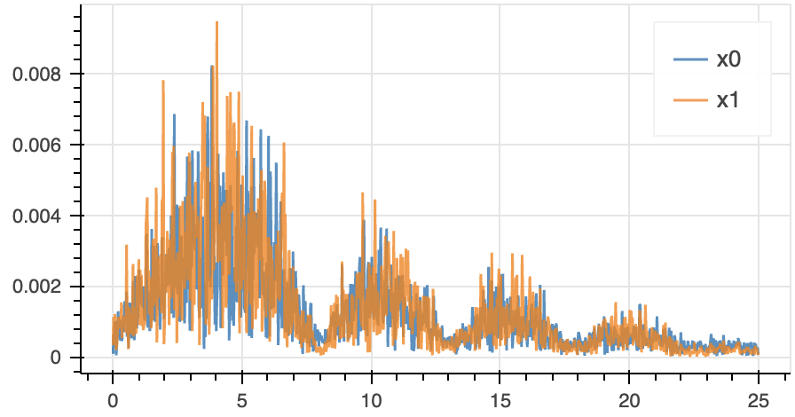
Residual FFT (frequency content)

Same residual, viewed as a frequency spectrum.

Residual FFT example

Residual FFT example.

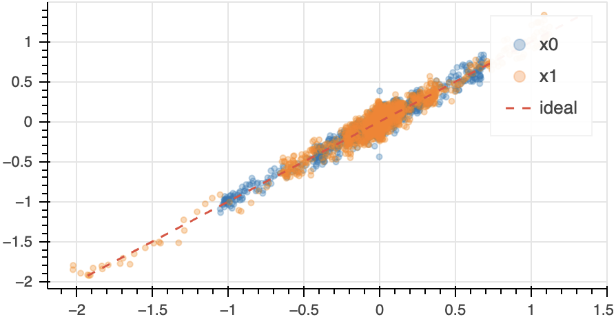
True vs. predicted derivative

Each point plots \( \dot{x}_{\text{predicted}} \) against \( \dot{x}_{\text{true}} \) for one sample.

True vs. predicted derivative

True vs. predicted derivative example.

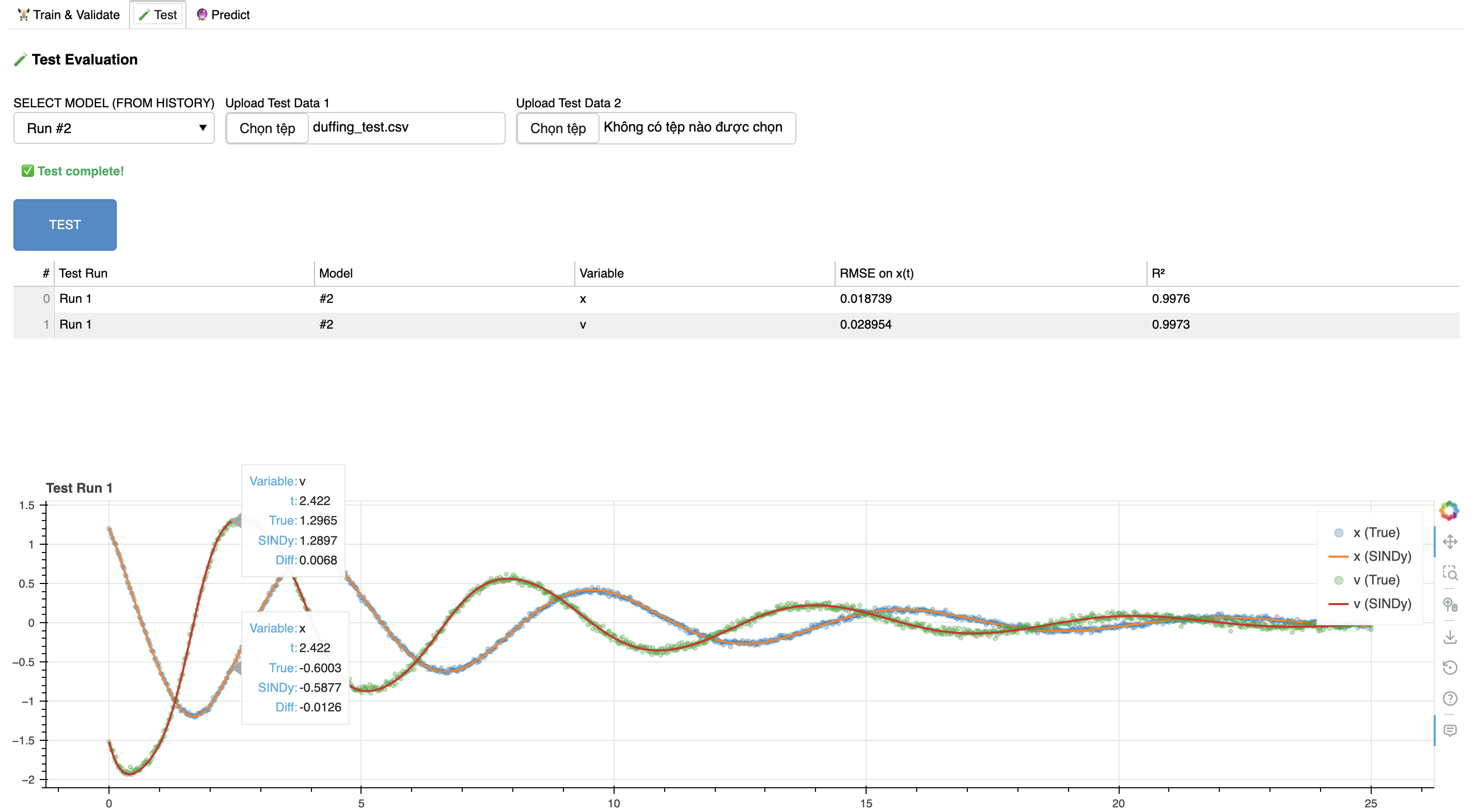
Pick a trained model and a held-out test trajectory, then press TEST — the discovered equations are forward-simulated from the test file's initial condition and compared against the real data. This checks whether the model actually generalizes, not just fits.

Test tab overview

The Test tab — model & data selectors, overlay plot, and metrics table.

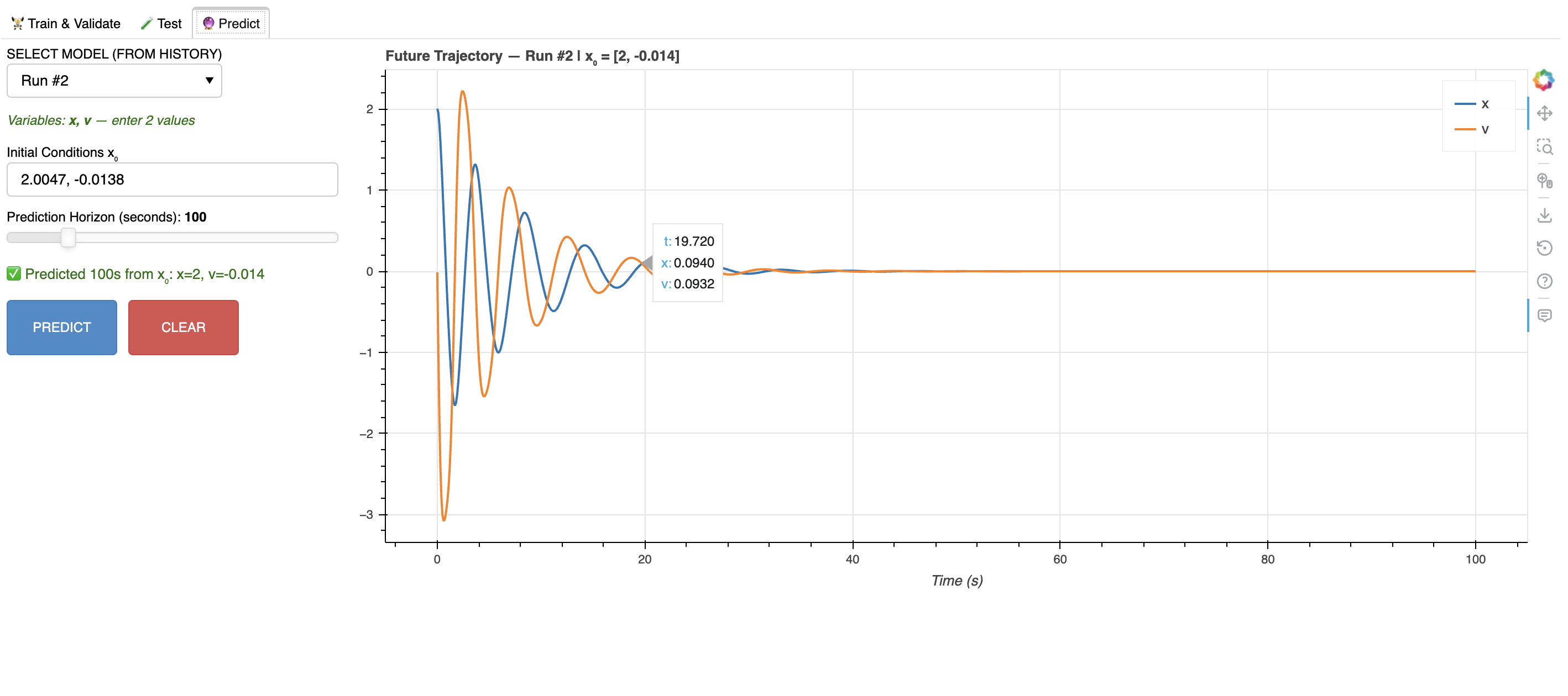
Pick a trained model, set a new initial condition and a time horizon, then press PREDICT — the discovered equations are simulated forward from that starting point, with no true trajectory to compare against. Use this to explore how the model behaves beyond your original data.

Predict tab overview

The Predict tab — model selector, initial condition & horizon controls, and the simulated trajectory plot.

Ask the SINDy Assistant

SINDy AssistantResearch workflow guide
Hi — I’m the SINDy Assistant.

Choose a question or search the curated knowledge base. I can explain this module’s workflow, metrics, predictions, and ensemble results.